Dynamic Portfolio Optimization Example
Portfolio optimization selects assets to balance return and risk. This dynamic variant extends classical Markowitz theory across multiple time periods and incorporates transaction costs when rebalancing portfolios.
In this formulation, asset selections are optimized jointly over all time steps. The model assumes that expected returns and risk estimates are known for each period, resulting in a globally optimal sequence of portfolio decisions.
This corresponds to an offline optimization setting (also referred to as perfect foresight), where future information is available during optimization. As such, the model provides a theoretical benchmark for multi-period portfolio allocation rather than a directly implementable trading strategy.
import getpass
import os
from datetime import datetime, timedelta

import pytz
import yfinance as yf
from dotenv import load_dotenv
from luna_quantum.algorithms import SCIP

from luna_usecases.dynamic_portfolio_optimization import (
    DynamicPoCollection,
    DynamicPoData,
    DynamicPoFormulation,
    DynamicPoInstance,
)

load_dotenv()
if "LUNA_API_KEY" not in os.environ:
    os.environ["LUNA_API_KEY"] = getpass.getpass("Enter your Luna API key: ")
Download Historical Market Data
We start by selecting a set of assets and downloading historical price data.
From these prices, we compute daily returns, which will serve as the basis for estimating: - expected returns - risk (covariance)
tickers = ["AAPL", "MSFT", "GOOGL", "AMZN", "TSLA", "JPM", "JNJ", "V"]
end_date = datetime.now(tz=pytz.timezone("Europe/London"))
start_date = end_date - timedelta(days=180)

stock_data = yf.download(tickers, start=start_date, end=end_date, progress=False)

close = stock_data["Close"]
daily_returns = close.pct_change().dropna()
returns = daily_returns.values  # shape: (T, N)
From Static Returns to Time-Dependent Estimates
In a static portfolio model, we would compute a single: - expected return vector μ - covariance matrix Σ
However, in a dynamic setting, these quantities change over time.
To model this, we estimate:
- μ[t]: expected returns at time step t
- Σ[t]: covariance matrix at time step t
using a rolling window over past observations.
Rolling Window Estimation
We use a rolling window of fixed size to estimate statistics from recent data.
For each time step t:
- we look at the last window observations
- compute the average return (μ[t])
- compute the covariance matrix (Σ[t])
This means that each estimate is based only on past observations relative to t.
However, note that in the subsequent optimization step, all time steps are considered jointly.
As a result, while the statistical estimates themselves do not use future data, the overall optimization still operates in an offline setting with access to all time steps simultaneously.
window = 10  # rolling window

data = DynamicPoData.from_returns(
    tickers=tickers,
    returns=returns,
    window=window,
    pick_n=3,
    risk_aversion=1.5,
    transaction_cost=0.01,
)
data = DynamicPoData(
    tickers=["AAPL", "GOOGL", "MSFT"],
    expected_returns=[[0.05, 0.08, 0.03], [0.06, 0.04, 0.07]],
    covariance_matrices=[
        np.array([[0.04, 0.01, 0.005], [0.01, 0.09, 0.02], [0.005, 0.02, 0.03]]),
        np.array([[0.05, 0.015, 0.01], [0.015, 0.07, 0.025], [0.01, 0.025, 0.04]]),
    ],
    n_assets=3,
    n_time_steps=2,
    pick_n=2,
    risk_aversion=1.0,
    transaction_cost=0.01,
)
print(data.to_string())
Plot Data
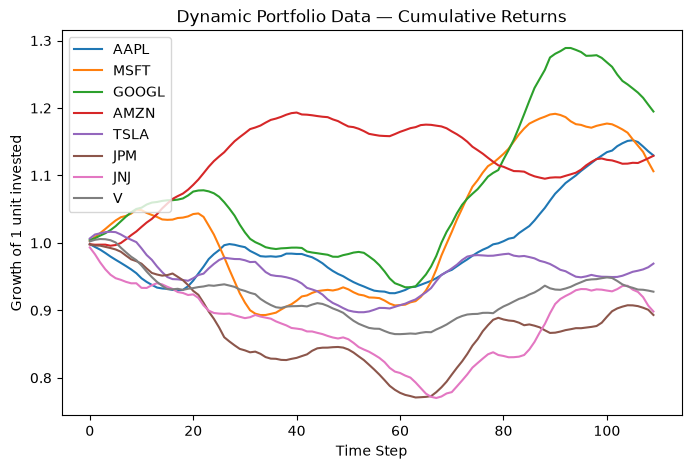
Visualize expected returns and risk across time periods.
<Axes: title={'center': 'Dynamic Portfolio Data — Cumulative Returns'}, xlabel='Time Step', ylabel='Growth of 1 unit invested'>
Create Formulation
Optimize multi-period asset allocation balancing returns, risk, and transaction costs.
Dynamic Portfolio Optimization Formulation:
  Assets: 8
  Time steps: 110
  Pick per period: 3
  Risk aversion: 1.5
  Transaction cost: 0.01

Decision Variables:
  x[t,i] in {0,1} for t = 0, ..., 109, i = 0, ..., 7
  x[t,i] = 1 if asset i is selected at time step t
  z[t,i] in {0,1} for t = 1, ..., 109, i = 0, ..., 7
  z[t,i] = 1 if asset i changes between t-1 and t
  Total: 1752 binary variables

Objective:
  maximize sum_t sum_i mu[t][i]*x[t,i]
           - risk_aversion * sum_t sum_{{i,j}} sigma[t][i][j]*x[t,i]*x[t,j]
           - transaction_cost * sum_{{t>0}} sum_i z[t,i]

Constraints:
  1. Pick exactly 3 assets per period (110 constraints):
     sum_i x[t,i] == 3  for all t = 0, ..., 109
  2. Transaction cost linearization (1744 constraints):
     z[t,i] >= x[t,i] - x[t-1,i]  for all t = 1, ..., 109, i = 0, ..., 7
     z[t,i] >= x[t-1,i] - x[t,i]  for all t = 1, ..., 109, i = 0, ..., 7
Create Instance
Combine data and formulation into a solvable instance.
Data:Dynamic Portfolio Optimization Data:
  Tickers: AAPL, MSFT, GOOGL, AMZN, TSLA, JPM, JNJ, V
  Number of assets: 8
  Time steps: 110
  Assets to select per period: 3
  Risk aversion: 1.5
  Transaction cost: 0.01
Formulation:Dynamic Portfolio Optimization Formulation:
  Assets: 8
  Time steps: 110
  Pick per period: 3
  Risk aversion: 1.5
  Transaction cost: 0.01

Decision Variables:
  x[t,i] in {0,1} for t = 0, ..., 109, i = 0, ..., 7
  x[t,i] = 1 if asset i is selected at time step t
  z[t,i] in {0,1} for t = 1, ..., 109, i = 0, ..., 7
  z[t,i] = 1 if asset i changes between t-1 and t
  Total: 1752 binary variables

Objective:
  maximize sum_t sum_i mu[t][i]*x[t,i]
           - risk_aversion * sum_t sum_{{i,j}} sigma[t][i][j]*x[t,i]*x[t,j]
           - transaction_cost * sum_{{t>0}} sum_i z[t,i]

Constraints:
  1. Pick exactly 3 assets per period (110 constraints):
     sum_i x[t,i] == 3  for all t = 0, ..., 109
  2. Transaction cost linearization (1744 constraints):
     z[t,i] >= x[t,i] - x[t-1,i]  for all t = 1, ..., 109, i = 0, ..., 7
     z[t,i] >= x[t-1,i] - x[t,i]  for all t = 1, ..., 109, i = 0, ..., 7
Formulate Model
Translate the instance into a mathematical optimization model.
Solve and Interpret
Solve the model with SCIP and interpret the raw result into a use-case-specific solution.
scip = SCIP()
job = scip.run(model)
sol = job.result()
uc_solution = instance.interpret(sol)
print(uc_solution.to_string())
/Users/maximilianjanetschek/PycharmProjects/luna-usecases/.venv/lib/python3.13/site-packages/rich/live.py:260:
UserWarning: install "ipywidgets" for Jupyter support
  warnings.warn('install "ipywidgets" for Jupyter support')
2026-06-16 21:16:44 INFO Sleeping for 5.0 seconds. Waiting and checking a function in a loop.
2026-06-16 21:16:51 INFO Sleeping for 10.0 seconds. Waiting and checking a function in a loop.
2026-06-16 21:17:04 INFO Sleeping for 15.0 seconds. Waiting and checking a function in a loop.
Dynamic Portfolio Optimization Solution:
  Status: VALID
  Period 0: MSFT, GOOGL, AMZN
  Period 1: MSFT, GOOGL, AMZN
  Period 2: MSFT, GOOGL, AMZN
  Period 3: MSFT, GOOGL, AMZN
  Period 4: MSFT, GOOGL, AMZN
  Period 5: MSFT, GOOGL, AMZN
  Period 6: MSFT, GOOGL, AMZN
  Period 7: MSFT, GOOGL, AMZN
  Period 8: MSFT, GOOGL, AMZN
  Period 9: MSFT, GOOGL, AMZN
  Period 10: MSFT, GOOGL, AMZN
  Period 11: MSFT, GOOGL, AMZN
  Period 12: MSFT, GOOGL, AMZN
  Period 13: MSFT, GOOGL, AMZN
  Period 14: MSFT, GOOGL, AMZN
  Period 15: MSFT, GOOGL, AMZN
  Period 16: MSFT, GOOGL, AMZN
  Period 17: MSFT, GOOGL, AMZN
  Period 18: MSFT, GOOGL, AMZN
  Period 19: AAPL, GOOGL, AMZN
  Period 20: AAPL, GOOGL, AMZN
  Period 21: AAPL, AMZN, TSLA
  Period 22: AAPL, AMZN, TSLA
  Period 23: AAPL, AMZN, TSLA
  Period 24: AAPL, AMZN, TSLA
  Period 25: AAPL, AMZN, TSLA
  Period 26: AAPL, AMZN, TSLA
  Period 27: AAPL, AMZN, TSLA
  Period 28: AAPL, AMZN, TSLA
  Period 29: AAPL, AMZN, TSLA
  Period 30: AAPL, AMZN, TSLA
  Period 31: AAPL, AMZN, TSLA
  Period 32: AAPL, AMZN, TSLA
  Period 33: AAPL, MSFT, AMZN
  Period 34: AAPL, MSFT, AMZN
  Period 35: AAPL, MSFT, AMZN
  Period 36: AAPL, MSFT, AMZN
  Period 37: AAPL, MSFT, AMZN
  Period 38: AAPL, MSFT, AMZN
  Period 39: MSFT, AMZN, JPM
  Period 40: MSFT, AMZN, JPM
  Period 41: MSFT, AMZN, JPM
  Period 42: MSFT, AMZN, JPM
  Period 43: MSFT, AMZN, JPM
  Period 44: MSFT, AMZN, JPM
  Period 45: MSFT, AMZN, JPM
  Period 46: MSFT, AMZN, JPM
  Period 47: MSFT, AMZN, JPM
  Period 48: MSFT, AMZN, JPM
  Period 49: MSFT, AMZN, JPM
  Period 50: MSFT, AMZN, JPM
  Period 51: MSFT, AMZN, TSLA
  Period 52: MSFT, AMZN, TSLA
  Period 53: MSFT, AMZN, TSLA
  Period 54: MSFT, AMZN, TSLA
  Period 55: MSFT, AMZN, TSLA
  Period 56: MSFT, AMZN, TSLA
  Period 57: MSFT, AMZN, TSLA
  Period 58: MSFT, AMZN, TSLA
  Period 59: MSFT, AMZN, TSLA
  Period 60: MSFT, AMZN, TSLA
  Period 61: MSFT, AMZN, TSLA
  Period 62: MSFT, AMZN, TSLA
  Period 63: MSFT, AMZN, TSLA
  Period 64: MSFT, GOOGL, TSLA
  Period 65: MSFT, GOOGL, TSLA
  Period 66: MSFT, GOOGL, TSLA
  Period 67: MSFT, GOOGL, TSLA
  Period 68: MSFT, GOOGL, TSLA
  Period 69: MSFT, GOOGL, JPM
  Period 70: MSFT, GOOGL, JPM
  Period 71: MSFT, GOOGL, JPM
  Period 72: MSFT, GOOGL, JPM
  Period 73: MSFT, GOOGL, JPM
  Period 74: MSFT, GOOGL, JPM
  Period 75: MSFT, GOOGL, JPM
  Period 76: MSFT, GOOGL, JPM
  Period 77: MSFT, GOOGL, JPM
  Period 78: MSFT, GOOGL, JPM
  Period 79: MSFT, GOOGL, JPM
  Period 80: AAPL, MSFT, GOOGL
  Period 81: AAPL, MSFT, GOOGL
  Period 82: AAPL, MSFT, GOOGL
  Period 83: AAPL, MSFT, GOOGL
  Period 84: AAPL, MSFT, GOOGL
  Period 85: AAPL, GOOGL, JNJ
  Period 86: AAPL, GOOGL, JNJ
  Period 87: AAPL, GOOGL, JNJ
  Period 88: AAPL, GOOGL, JNJ
  Period 89: AAPL, GOOGL, JNJ
  Period 90: AAPL, GOOGL, JNJ
  Period 91: AAPL, JPM, JNJ
  Period 92: AAPL, JPM, JNJ
  Period 93: AAPL, JPM, JNJ
  Period 94: AAPL, JPM, JNJ
  Period 95: AAPL, AMZN, JPM
  Period 96: AAPL, AMZN, JPM
  Period 97: AAPL, AMZN, JPM
  Period 98: AAPL, AMZN, JPM
  Period 99: AAPL, AMZN, JPM
  Period 100: AAPL, AMZN, JPM
  Period 101: AAPL, AMZN, JPM
  Period 102: AAPL, AMZN, JPM
  Period 103: AAPL, AMZN, JPM
  Period 104: AAPL, AMZN, JPM
  Period 105: AMZN, TSLA, JPM
  Period 106: AMZN, TSLA, JPM
  Period 107: AMZN, TSLA, JPM
  Period 108: AMZN, TSLA, JPM
  Period 109: AMZN, TSLA, JPM
  Portfolio Return:   1.456639
  Portfolio Risk:     0.115417
  Transaction Costs:  0.240000
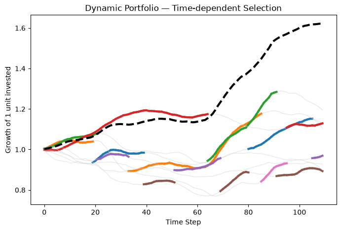
Plot Solution
Visualize the optimal solution.
<Axes: title={'center': 'Dynamic Portfolio — Time-dependent Selection'}, xlabel='Time Step', ylabel='Growth of 1 unit invested'>
Collections
Generate a benchmark collection of random instances for batch processing.
collection = DynamicPoCollection.from_random(
    min_assets=3, max_assets=6, n_time_steps=2, pick_n=2, num_instances=1, seed=42
)
model = collection.instances[0].formulate()
print(model)
Model: dynamic_portfolio_optimization<s42_n3_i0>
Maximize
  -0.00031845908234652613 * x_0_0 * x_0_1 - 0.005378824097872742 * x_0_0 * x_0_2
  - 0.003801733038977486 * x_0_1 * x_0_2 + 0.006563805484193941 * x_1_0 * x_1_1
  - 0.006438512615851617 * x_1_0 * x_1_2 - 0.006590377259410821 * x_1_1 * x_1_2
  + 0.03303333549964048 * x_0_0 + 0.013952958333736984 * x_0_1
  + 0.052749880094328724 * x_0_2 + 0.03631039904708676 * x_1_0
  + 0.021702789925954542 * x_1_1 + 0.04562590629288803 * x_1_2 - 0.01 * z_1_0
  - 0.01 * z_1_1 - 0.01 * z_1_2
Subject To
  pick_n_period_0: x_0_0 + x_0_1 + x_0_2 == 2
  pick_n_period_1: x_1_0 + x_1_1 + x_1_2 == 2
  tc_pos_1_0: x_0_0 - x_1_0 + z_1_0 >= 0
  tc_neg_1_0: -x_0_0 + x_1_0 + z_1_0 >= 0
  tc_pos_1_1: x_0_1 - x_1_1 + z_1_1 >= 0
  tc_neg_1_1: -x_0_1 + x_1_1 + z_1_1 >= 0
  tc_pos_1_2: x_0_2 - x_1_2 + z_1_2 >= 0
  tc_neg_1_2: -x_0_2 + x_1_2 + z_1_2 >= 0
Binary
  x_0_0 x_0_1 x_0_2 x_1_0 x_1_1 x_1_2 z_1_0 z_1_1 z_1_2